Hello everyone, another computer vision blog here. Computer vision is a very interesting topic to me because in my opinion, images hold a lot of information related to a robots operating environment. While the theme of computer vision has a lot subtopics one could cover, the one I’d like to focus on is the concept of feature tracking. Before we start I’d like to take a quick step back and break down the key steps required in a feature tracking pipeline.

Image Features, what are they?

Raw camera images contain a lot of information, but this can also be a downside because prior to using an images to perform a specific task we need to identify what it is in the image that we are interested in. There are an incredible numbers of ways to process an image such as a color threshold, if we only want to track a specific color in an image, to filtering by shapes using blob detection. In an autonomous driving application an image can be filtered using a Sobel filter ( If you want more information this is a good place to start https://en.wikipedia.org/wiki/Sobel_operator) which can help extract and emphasize clear edges in an image.

This can be a first step in identifying the lanes in a road which we want to follow. Another useful technique is called Harris corner detection ( Again this would be a good place for more in depth information https://en.wikipedia.org/wiki/Harris_corner_detector) we can extract corners in an image if we have some prior knowledge that our environment may have some clear edges we want to keep track of.

In my quick exploration I also wanted to use a Harris corner detector as I knew the images being looked at had sharp corners I could use as features to follow. In OpenCV the function goodFeaturesToTrack gives you access to the Schi-Thomasi corner detector which was a modification made to the Harris Corner detector by extracting points strongly related to corners in an image.

Depending on the images processing application you’d like to use, you may have a completely different way of defining what a feature is. More advanced examples of images features include SIFT which can give you more detailed information about features in an image (Rather than just the pixel coordinates like the Schi-Thomasi corner detector). You may also use a Neural Network based feature detector to detect objects of interest and then apply optical flow to identify how fast they are moving from one frame to another.

I have features, what’s next?

Once you have found a feature you’d like to track you’ll need to find a method of quantifying the displacement of the markers from one image to another. This is where the concept of optical flow comes into play.

Optical flow is the idea of estimating the motion of a pixel across a sequence of images. Optical flow usually has 2 main implementations, one which looks a the entire image (global optical flow) or at key points in an image (sparse optical flow).

A pixel’s value can be described as a function of it’s x and y coordinate as well as time t. An assumption made is that for a pixel moving along x and y for a time change dt, the intensity is the same. This generates an equation which relates the gradients of a pixel ( in the x, y and t directions) as wells as pixel velocities Vx and Vy.

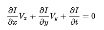
The partial derivatives are flow fields which describe the motion of a pixel’s intensity with respect to the x and y coordinates. These field’s can also be plotted for easy visualization. The problem with this equation is that the velocities Vx and Vy are unknown but we only have one pixel to use as a refernce which makes our equation under defined. There are great resources out there which explain the optical flow algorithm in more technical detail, good starting points I’d suggest are:

• OpenCV: Optical Flow
• Computer Vision Algorithms and Applications by Richard Szeliski (Recommended during my Unmanned Autonomous Systems class at UofT)
• Robotics, Vision and Control by Peter Corke (This resource goes into a lot of detail in what’s required to solve the optical flow problem and the image intensity constraint I mentioned above).

Lucky, OpenCV has a function which implements the Lucas-Kanade method for solving the optical flow equation. The function calcOpticalFlowPyrLK uses a set of reference pixels, a previous image and current image to output a sequence of pixels based on the motion from the previous time step to the current one.

Putting it all together

My next step, now that I have a pipeline for visualizing the motion of pixels in an image, was to apply it on a dataset. In my case I used a sample dataset from the Oxford robocar dataset to apply some image processing on a set of grayscale images at the front of a vehicle. The dataset can be found at https://robotcar-dataset.robots.ox.ac.uk/ The result of my quick project was the following:

This implementation is great for visualizing the pixel displacement in an image but this is all done in the image frame. To integrate this in an autonomous stack I’d also want to consider the motion of the pixels in the vehicle frame. To do this I need to consider the camera intrinsic parameters. These are static and are related to the senor used in the camera. The next step is the camera extrinsic parameters, that is, the location and orientation of the camera with respect to the centroid of my car.